Agisoft Photoscan¶

Initial Set Up¶

This section is necessary when it is your first time using Agisoft on a given computer. Once you have set everything up the way you want it, Agisoft will save your preferences. Let’s get started!

Make a folder in Photoscan or Pix4D with the generalized name of the Flight example “RR_20180613”

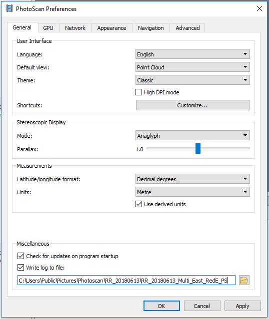
Set the working directory and the name of the files that will be written within it. Tools > Preferences

File > Save As

Documents that will make your life easier

1. A CSV that lists your Ground Control Points (GCP) that you collected from the field with a label, latitude, longitude, and altitude. Altitude is used for the DSM and Point Cloud generation.
2. A CSV with the specific calibration panel reflectance values for each wavelength

• MicaSense: RP04-1806002-SC
• MicaSense: RP02-1603210-SC
• MapIR: Version 1

Implementing Documents

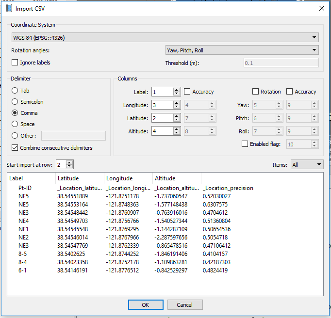
Go to reference tab at the bottom of the left window and then hit the folder icon on the top left. Go to the cleanedGCP folder and select. Make sure you’re in the correct coordinate system. Under Delimiter, select the Comma option. Under the columns, make sure to select the box that says Accuracy, next to the initial label box.

Created new project¶

When starting a new project it is best to set all of the working paths initially. First we are going to save the project. Here we will give it the appropriate name and set the directory. Next we will set the working directory for all the created documents by setting our preferences. Then we can add the images from the flight and the calibration as well as the csv with the desired gcp coordinates.

File > Save As… > change the project title > OK

Tools > Preferences > edit the end of the extension > OK

Example:

Workflow> add images> (select images)>Open> create for multispectral

Workflow> add images> (add calibration panel images [all bands]) > Open> create for multispectral

Add the images of the flight as well as the calibration images. The images from the calibration should be put into a separate folder automatically. I the left hand window there are two tabs you can select: Workspace and Reference…. Select the “Reference” tab and continue.

>add cvs of gcps > Click “Yes to All”

Now, we can align the photos. This will estimate where the ground control points are in relationship to the images.

Workflow > align photos…. > High > OK

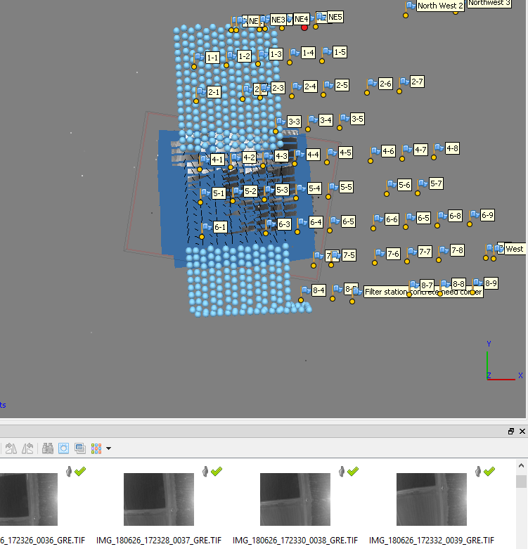
I like to uncheck the gcps that are not relevant and it looks like this:

GCPs:¶

Pro Tip: You can reduce the time you spend looking through irrelevant GCPs when you have GCPs throughout a large area and you only need to use a section of them by unchecking irrelevant GCPs using the “Model” tab in combination with the GCP list in the lower left window.

Right click on a GCP in the lower left window > filter photos by markers.

This will show the images that it thinks has the gcp in view in the lower right window. Double click on one of these images from the lower right hand window (Under the Photos tab) to open the view in the upper right window. Move the marker to the correct location in the appropriate photos. This will make a green flag on the points that you set.

Pro Tip: After you do this to two of the images you can filter the images again and reduce to images that actually have the GCP in it.

Repeat moving markers for as many photos as necessary, approximately 6 but up to you.

Camera calibration:¶

Tools > Camera Calibration… > Bands (tab) > check “Normalize Sensitivity”

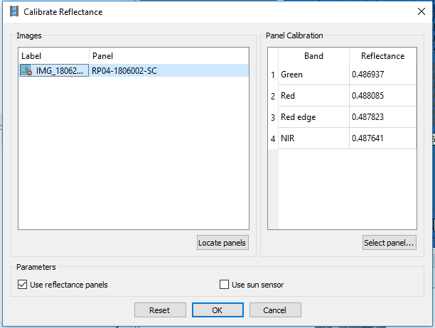
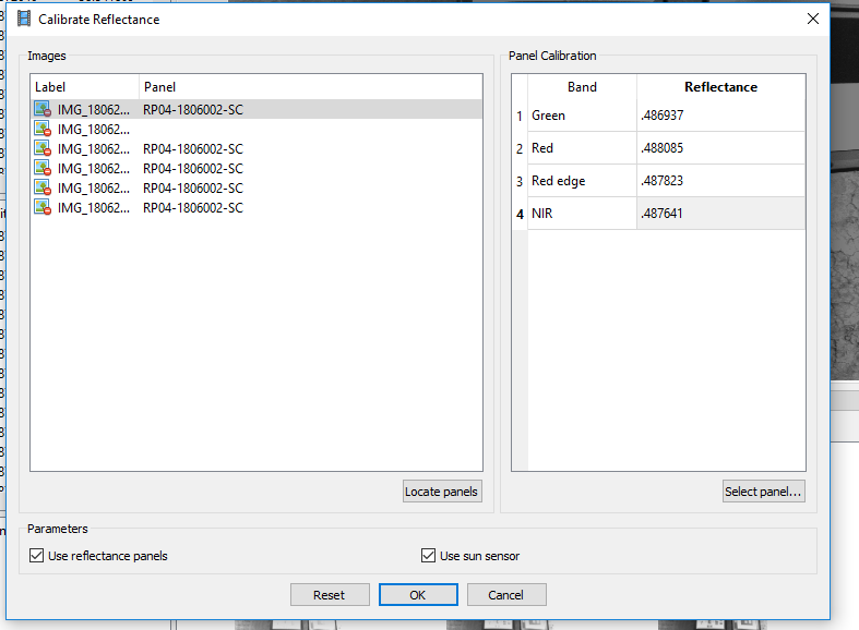
Tools > Reflectance Calibration… > locate bands> select at least one from the list on the left window. > Select the box to “Use reflectance panels” and if you used a sun sensor you can select “Use sun sensor” > OK

Don’t Panic! Your images may adjust to a different color. In this demonstration everything turned very dark, almost black. The quick fix is to adjust the brightness to an appropriate level. Recommendation of 500%.

Then on the right side of this window ensure that the reflectance values are correct. If necessary select “Select Panel” and add the csv of the band values. The value in the right window may need to be in this format: 0.48756. If the decimal is in the tenth place then you can adjust these values manually by double clicking on them.

Ensure that each band of the calibration images has the reflectance square properly highlighted. Most of the time the software will not have a problem reading these in as long as the QR code is visible in the image. If there is an issue you may need to select the squares manually.

Tools > Select Primary Channel > Select from drop down > Apply. Repeat process for all images.

Normally, If one is found then all will be set correctly but safe to check.

Pro Tip: set the primary channel to a band that is easy for you to see the details of the image in like the red band. This will help when you are doing GCPs.

Optimize camera alignment:¶

This is one of the easiest steps. Once you have completed your ground truthing of the GCPs you can press . This will correct the location of all of your photos in relationship to each other and the ground control points. Select “OK” to the default selection.

Build Dense Cloud:¶

Workflow > Build dense cloud…

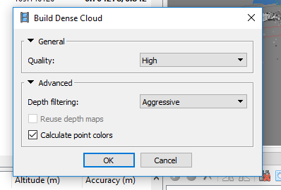
Build Mesh:¶

Workflow > Build Mesh > Select the “Source Data” to be the “Dense Cloud” that we just created > OK

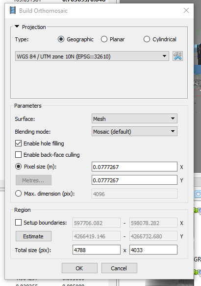
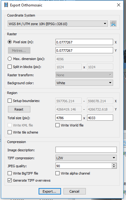
Build Orthomosaic:¶

We want our output projection in WGS 84/UTM zone 10N for this specific project. Select the drop down arrow and if you do not see the output projection you want select “More…” and search in this window for the one you would like.

Select “Estimate” then hit “OK”.

Export Orthomosaic:¶

File > Export > Export Orthomosaic > Export JPEG/TIFF/PNG… > (Check settings) Export….

Normalize values and Generate Preview¶

One of the issues that we ran into when using Photoscan is the distribution of values comes out between 0 and 65535 and we want it to be between 0 and 1. We can this normalizing. We wrote a code in R to to do this for us.

You will need:

1. RStudio
2. Project Folder with the codes in it.
3. Script: “post-process.R”

First, right click on the TIFF file that you just made when you exported the orthomosaic and select “Copy” this is going to copy the file path to this tiff. Open R studio and use the following set up:

1. Run the library and the three sources
2. In the console, assign “ortho” to the path that you just copied by right clicking and selecting “Paste” Note that it should be in quotations and the beginning part has been deleted. Also, either / or \\ for the directory will work in R.
3. Then, run the lines 31 to 64 (may be subject to change). Otherwise from the first “if” statement to the end of the script.

• The first “if” statement does not need to be run. It is a contingency for if ortho was assigned a folder from Pix4D.
• The second “if” statement is normalizing the reflectance to be values between 0 and 1.
• The last “if” statement is creating the preview .png based on the number of bands the image has.

1. Now look in the folder where your original tiff is. The new tiff and png will have “_reflectance.tif” as the ending.

Processing Report¶

This is an option that is nice to have and simple to do.

File > Export > Generate Report > the title of the report can be changed here > OK > choose directory and name of the file. Example: “processing-report” > Choose file type. PDF preferred > Save

Uploading Data¶

You can either use the Google Drive Internet interface to upload the documents or you can use the Google drive file stream in the file explorer interface. The Google file stream seems to work more reliably.

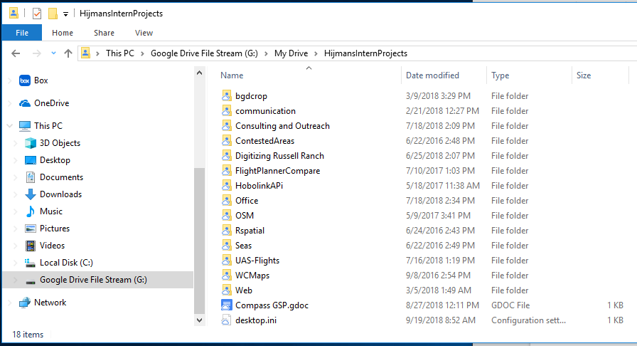
Files that need to be uploaded: One copy of everything to the flight folder in a project folder. Example: HijmansInternProjects\UAS-Flights\RussellRanch\Flight Data\2018-06-26\East\PS

One copy of the final normalized tiff and the png to the results folder. Example: HijmansInternProjects\UAS-Flights\RussellRanch\Flight Data\Results\Multi Merged Reflectance